As you all know, number 0 only exists in Excel file through a certain calculation result. However, it does not support anything in your calculation, but also contributes to make our data more gloomy 😀
Therefore, to identify the source of the lack of such positive. Today I will share with you 3 ways to hide a value of 0 in Excel the fastest.
Okey, we will go into the detailed tutorial now!
Read more:
Method # 1. Remove zero values with Format Cells
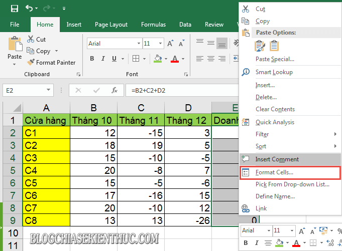
+ Step 1: First you open the Excel file to be processed. Here you select / highlight the data to be hidden 0 => Then right click and select Format Cells.
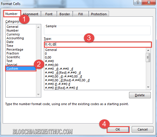
+ Step 2: Dialog box Format Cells opens => here you switch to tabs Number => and select Custom => then enter the command line 0;-0;;@ on item Type => Then press OK.
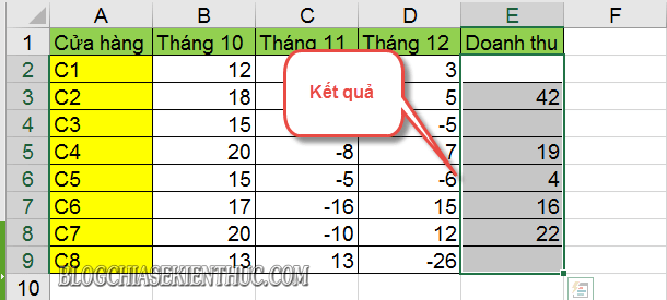
+ Step 3: Immediately, the results are equal 0 Excel worksheet has been hidden as shown below.
Method # 2. Eliminate a value of zero with Conditional Formatting
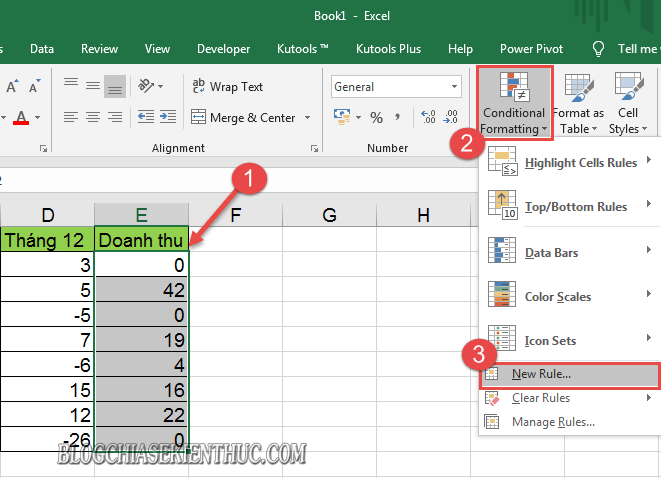
+ Step 1: Similar to how to filter numbers 0 In Method 1, you also need to create a selection for the worksheet value => and then click Conditional Formatting => and select New Rule.
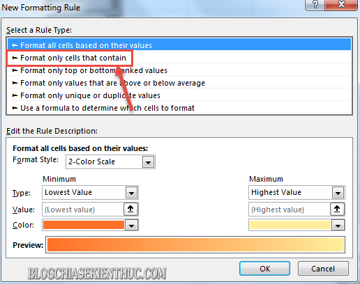
+ Step 2: Dialog box New Format Rule appears => here you click Format only cells that contain.
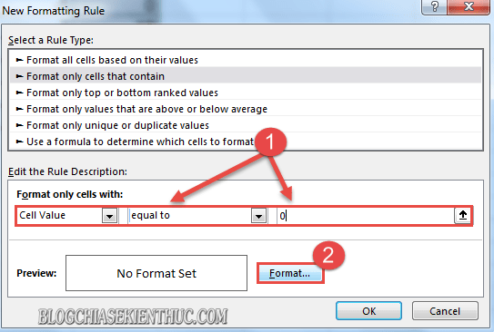
+ Step 3: And in the next dialog, set it up in the section Format only cells with respectively:
- Value Cells
- equal to
- And set the value to is 0 same picture
=> Then continue to press Format..
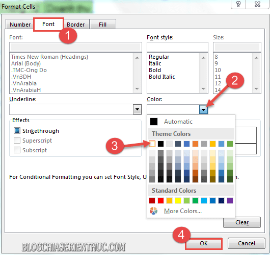
+ Step 4: Then open the tab Font at the dialog box Format Cells, you set Color is the moon color => and click OK to apply.
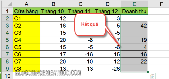
And finally we get the results as shown below.
Method # 3. Automatically remove zero values right on the Sheet
Different from the two ways of filtering values (number 0) as above, with the number filtering method 0 On the Sheet you will only need to set once and from the next onwards when entering additional values to return numbers 0 In Sheet, Excel will automatically filter the value by 0 that does not take time to format each piece of data.
+ Step 1: You click on the menu ![]()
Options.
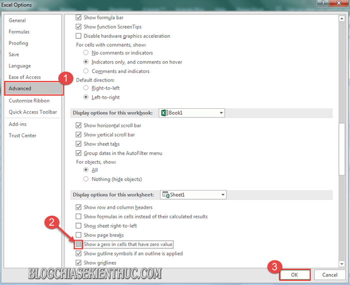
+ Step 2: Dialog box Options opens => here you switch to tabs Advanced => and then scroll down to the item Display options for this Wooksheet => and deselect at Show a zero in cells that have zero value.
=> Then press OK to set hidden values equal to 0 on Sheet.
# 4. Epilogue
Okay, so I just gave you very detailed instructions 3 ways to hide zero values in Excel Alright then.
And here, my article would like to pause. Hope this tip will be helpful to you. Good luck !
CTV: Luong Trung - Blogchiasekienthuc.com
Note: Was this article helpful to you? Do not forget to rate the article, like and share it with your friends and relatives!

0 Comments